When you use a statistical model to generate a 12-month forecast, you get more than just twelve numbers. You also get a great deal of information about how the forecast was generated, the model’s fit to the historic data and different measures of expected forecast accuracy. In this article, we dissect and catalogue the different components of a statistical forecast.

Figure 1
The graph above contains three components, the demand history, the point forecasts and the confidence limits. Let’s consider each in turn.
Demand History
The green line represents the historic demand for instant cameras on a monthly basis. This type of data set, consisting of equally-spaced observations in time, is referred to as a time series. A forecasting technique which generates a forecast based solely on an item’s past demand history is referred to as a time series method. Typically, time series methods will capture structure such as current sales levels, trends and seasonal patterns, and extrapolate them forward.
Point Forecasts
The red line represents the point forecasts and the blue lines represent the associated confidence limits. The future is uncertain and a statistical forecasting model represents uncertainty as a probability distribution. The point forecast is the mean of the distribution and the confidence limits describe the spread of the distribution above and below the point forecast.
The point forecast can be thought of as the best estimate of the future. It is the point at which (according to the model) it is equally likely that the actual value will fall above or below. If we are trying to estimate expected revenue for our instant cameras, this is exactly what we want. We can take our point forecasts, and multiply by our average selling price to calculate our expected revenues.
Confidence Limits
On the other hand, suppose we want to know how many instant cameras we should stock. There are costs associated with carrying too much stock (e.g., warehousing, obsolescence, etc.) and there are costs associated with not carrying enough stock (e.g., lost sales, rush orders, etc.). This is where the confidence limits come into play. The confidence limits are calibrated to percentiles. In the example above, the upper confidence limit is set to 97.5% and the lower confidence limit is set to 2.5%. This means that (according to the model) the probability of future sales being at or below the upper confidence limit is 97.5% and the probability of future sales being at or below the lower confidence limit is 2.5%. Thus, if our desire is to maintain a service level of 97.5% we would stock to the upper confidence limit. Of course, Forecast Pro allows you to set the percentiles for the confidence limits to whatever values you desire.
Using the values of 2.5 and 97.5 for the lower and upper confidence limits is not uncommon. If you think about these settings for a minute, you will realize that the chances of the future sales falling in between these upper and lower bounds is 95%. Some people call this symmetric combination of upper and lower confidence limit settings the 95% confidence interval.

Figure 2
Consider the two graphs above. The graph on the left is the same as Figure 1 with the exception that we’ve added the fitted values. The fitted values show how the forecasting model “tracks” the history and can provide insight into how well the model captures the structure in the data.
Consider the graph on the right. Here we are using a best fit line to forecast the instant camera sales. As you may recall from your childhood schooling, the equation for a straight line is Y = mX + b , where m is the slope of the line, X is time and b is the intercept. Once we have selected m and b, this equation can be used not only to generate the forecasts, but also to fit the historical data. The graph on the left uses an exponential smoothing model to generate the fitted values and forecasts. Although the equations for the exponential smoothing model are more complex than for a straight line, the calculation of the fitted values and forecasts are performed in a similar fashion.
When we ask ourselves which of the two forecasting models depicted in Figure 2 is likely to forecast sales of instant cameras more accurately, the answer is clearly the exponential smoothing model. Why? Because it fits the historic data better.
In addition to examining the fitted values graphically, you can also calculate statistics to measure how closely they track the historic data. You can learn more about these in the Forecasting 101 post “A Guide to Forecast Error Measurement Statistics and How to Use Them.”
About the author:
 Eric Stellwagen is the co-founder of Business Forecast Systems, Inc. and the co-author of the Forecast Pro software product line. With more than 27 years of expertise, he is widely recognized as a leader in the field of business forecasting. He has consulted extensively with many leading firms—including Coca-Cola, Procter & Gamble, Merck, Blue Cross Blue Shield, Nabisco, Owens-Corning and Verizon—to help them address their forecasting challenges. Eric has presented workshops for a variety of organizations including APICS, the International Institute of Forecasters (IIF), the Institute of Business Forecasting (IBF), the Institute for Operations Research and the Management Sciences (INFORMS), and the University of Tennessee. He is currently serving on the board of directors of the IIF and the practitioner advisory board of Foresight: The International Journal of Applied Forecasting.