Forecasting is a dynamic and interdisciplinary field that involves a multitude of people, processes and techniques. Forecasters are constantly building on their current pool of knowledge in order to improve their processes, drawing on whatever resources they can find. A forecaster’s best resource, however, is often other forecasters—but it can be difficult to share information if everyone is speaking a different language. For this post we’ve compiled and defined a list of terms that every forecaster should be familiar with.
Keep in mind that some of these definitions are just brief introductions to larger concepts! Forecast Pro’s website and YouTube channel offer a wealth of resources that dive much deeper into forecasting techniques and terminology.
Working with Others
Forecasting is often one component within a larger planning process. As companies strive to increase transparency among the ongoing processes within their organizations, it is important to understand how the demand forecast fits into the larger picture.
Demand Consensus
Forecasting is often performed in a collaborative setting. Though the specifics of these processes vary, the ultimate goal is to come to a demand consensus, where all parties involved agree on the final forecasts so the numbers can get passed on to the next step in the demand planning process.
Domain Knowledge
As helpful as a statistical forecast can be to predicting the future, a statistical forecasting model generates forecasts based solely on the numeric properties of a set of numbers. When preparing a forecast, the forecaster must also use his or her knowledge of the company’s products and services, their industry and other relevant information that may impact the future. This relevant information that a person possesses, but is not being captured in the statistical model, is referred to as domain knowledge.
Sales and Operations Planning (S&OP)
S&OP is an integrated business management process where different functional areas of an organization (e.g., sales, operations and executive management) strive to effectively coordinate their simultaneous processes in order to work toward the company’s common goals. Its proper execution requires a series of steps and meetings that help people understand the company’s current performance, disseminate information across functional areas and improve future actions and results. The generation of a baseline demand forecast is often a first step in the S&OP process.
Forecasting Models
 There are many different forecasting techniques in the literature and in use at organizations around the globe. In this section we’ll introduce a couple of general modeling terms and cover the more commonly applied forecasting models.
Statistical Forecasting Model
A statistical forecasting model is an equation or series of equations that capture patterns and relationships in historic demand data and/or external data. The forecasts are based on these patterns.
Time Series Models
Time series models are a subset of statistical forecasting models that base the forecast solely on the demand history of the item you are forecasting. They work by capturing patterns in the historical data and extrapolating them into the future. They are appropriate when you can assume a reasonable amount of continuity between the past and the future.
Exponential Smoothing Models
Exponential smoothing is a widely used time series forecasting technique. The models estimate and forecast the level of the data along with different types of trends and seasonal patterns. The models are adaptive, and when generating the forecasts give greater emphasis to the recent history versus the more distant past.
Event Models
Event models extend exponential smoothing models by allowing you to adjust for events such as product promotions, moveable holidays, business interruptions and other irregular occurrences. The input for an event model is both the historic demand for the item to be forecasted and a schedule listing the timing of any events that have occurred historically and (if applicable) the timing of any future events that will occur in the forecast period.
ARIMA Models (Box-Jenkins)
ARIMA models are a family of statistically sophisticated forecasting models popularized by George Box and Gwilym Jenkins. In business applications, the models are usually applied in univariate form (i.e., as time series models), however, multivariate forms also exist in the literature. Studies have shown that ARIMA models can yield superior forecasts to exponential smoothing models for certain types of data and less accurate forecasts for other types of data. The ARIMA acronym stands for “AutoRegressive Integrated Moving Average” and many forecasters refer to ARIMA models as “Box-Jenkins models”.
Regression Models (and Dynamic Regression Models)
In contrast to time series forecasting, where past patterns are used exclusively to generate the forecasts, regression models allow you to incorporate explanatory variables such as prices, promotions and measures of the economy into the model. The most basic form of regression is known as ordinary least squares (OLS) and is available in many applications including Excel. Advanced regression models that combine time series approaches with the inclusion of explanatory variables are known as dynamic regression models and are available in specialized forecasting applications such as Forecast Pro XE.

Bottom-up and Top-down Forecasting
When preparing forecasts for hierarchical data, you must decide upon a reconciliation strategy (i.e., you must decide how to enforce that the forecasts are consistent across levels). One approach is to apply statistical forecasting methods directly to the lowest-level demand histories and construct all group-level forecasts by summing the lower-level forecasts—this is known as a bottom-up forecast. An alternative approach is to use statistical forecasting methods on more aggregated data and then to apply an allocation scheme to generate the lower-level forecasts—this is known as a top-down forecast.
Modeling Terms
There are a variety of terms that are used to describe inputs and outputs from statistical forecasting models. In this section we’ll cover a few of them.
Point Forecast
The point forecast is a number representing an estimate of demand at a future point in time. If the point forecast is generated using a statistical model then generally it will represent the mean value of the distribution of future values. This can be thought of as the point at which, according to the model, the future value is equally likely to fall above as below.
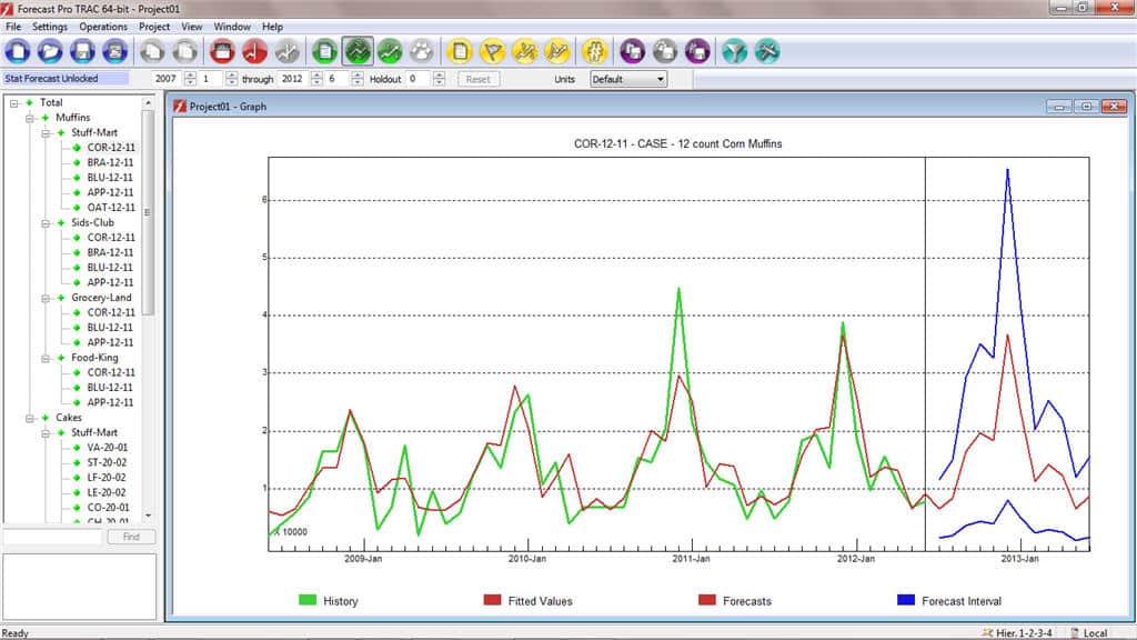
Confidence Limits (Prediction Intervals)
Confidence limits (also known as prediction intervals) are an indication of the uncertainty surrounding the point forecasts. Statistical forecasting models generally produce point forecasts along with upper and lower confidence limits. Each confidence limit is associated with a certain percentile. If the upper confidence limit is calculated for 97.5% and the lower for 2.5%, then according to the model, the actual values should fall below the upper confidence limit 97.5% of the time, and below the lower confidence limit 2.5% of the time. These specific settings for the upper and lower confidence limits (97.5% and 2.5% respectively) are often called the 95% confidence limits to indicate that the actual values should fall within the confidence limits 95% of the time. In practice, confidence limits tend to overstate accuracy.
Coefficients (Parameters)
Coefficients or parameters are numbers that go into a statistical forecasting model’s equations. Typically their values are either optimized to fit the data or set by the user. Coefficients control such things as rates of change, sizes of trends, response to explanatory variable, etc. As such, their values directly change both the forecasts and fit of the statistical model.
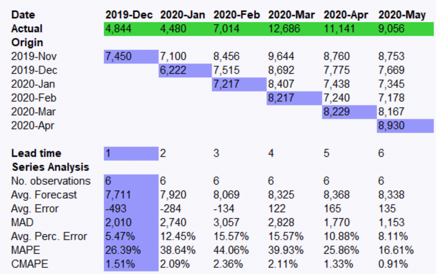
Lead Time
The Merriam Webster Dictionary defines lead time as, “The time between the beginning of a process or project and the appearance of its results”. In the context of statistical forecasting, the lead time refers to the number of periods ahead of the forecast origin (last historic data point) the forecast was made for. Thus, a one-month-ahead forecast would have a lead time of one, a two-month-ahead would be a lead time of two, etc.
Safety Stocks
Safety stock is the inventory needed above and beyond the forecast to mitigate the risk of running out of stock. Safety stocks can be set different ways including using the statistical forecasting model to estimate the expected variation from forecast, via simulation, using a policy such as days of inventory or specified minimum stocks.
Outliers
An outlier is a data point that falls outside the expected range of the data. If you are forecasting a time series that contains a significant outlier, there is a danger that the outlier could have a significant impact on the forecast.
Measuring Error
Error measurement is a critical component of key operations like building statistical forecasting models, tracking the accuracy of your forecasts, monitoring for exceptions and benchmarking your forecasting process. In this section we’ll review terms associated with measuring error.
Within-Sample vs. Out-of-Sample Statistics
Within-sample statistics measure the goodness-of-fit of the current statistical model to the historical data (i.e., how well the model tracks the historic data used to build it). Out-of-sample statistics measure how a forecast performed vs. what actually happened. Within-sample fit is almost always better than actual (out-of-sample) forecasting performance.
MAPE
The MAPE (Mean Absolute Percent Error) measures the size of the error in percentage terms. It is calculated as the average of the unsigned percentage error. Many organizations focus primarily on the MAPE when assessing forecast accuracy.
MAD
The MAD (Mean Absolute Deviation) measures the size of the error in units. It is calculated as the average of the unsigned errors.
R-Square
The R-square, or coefficient of determination, is a within-sample “goodness of fit” statistic that measures the fraction of variance explained by the model. For example, an R-Square of 0.79 indicates that the current model is explaining 79% of the overall variation in the data.
Summary
In the world of forecasting, there is constant room for improvement. Exchanging wisdom and information only serves to better your forecasting process, so we have presented this list of key terms to help make it easier for you to share information with fellow forecasters. For more resources on business forecasting, be sure to check out our other blog posts as well as our webinar archive on the Forecast Pro YouTube channel.